Step 1. Why Visualizing?
사람은 머신러닝 문제를 이해할 수 없습니다. 머신러닝 문제가 별로 복잡하지 않아도 사람은 머신러닝을 완벽하게 이해할 수 없습니다. 이는 사람이 태생적으로 가진 핸디캡이 있기 때문입니다.
사람은 3차원 공간에서 살고 있습니다. 3차원 공간 속에는 2차원, 1차원도 존재합니다. 우리가 보고 느낄 수 있는 것들은 1, 2, 3차원입니다. 하지만 머신러닝에서 다루는 차원의 수는 정말 큽니다. 많은 경우에서 훈련 샘플 각각은 수천 심지어 수백만 개의 차원을 가지고 있습니다.
이렇게 너무많은 차원은 사람이 머신러닝을 이해할 수 없게 만듭니다. 그래서 사람은 고차원을 저차원으로 변환하는 기술을 연구하였습니다. 이를 차원축소(Dimensionality Reduction)라고 합니다. 이러한 기술을 통해서 사람은 머신러닝을 더 직접적으로 잘 이해할 수 있게 됩니다.
차원축소(Dimensionality Reduction)를 수행하기 위해 MNIST dataset을 이용해봅니다.
Step 2. MNIST
MNIST는 가장 간단한 이미지 데이터셋입니다. 이 데이터셋은 $ 28 \times 28 $ pixel의 숫자 이미지로 구성되어있습니다. 실제로 데이터를 불러와서 확인해봅니다.
import numpy as np
import pandas as pd
import matplotlib.pyplot as plt
from sklearn.datasets import fetch_openml


mnist = fetch_openml('mnist_784', cache=False)
불러온 데이터를 이미지와 그 숫자가 무엇인지 알려주는 label로 나누어줍니다.
X = mnist.data.astype('float32').to_numpy()
y = mnist.target.astype('int64').to_numpy()
이미지 하나를 선택해봅니다.
plt.figure(figsize=(5,5))
idx = 5

grid_data = X[idx].reshape(28,28)  # reshape from 1d to 2d pixel array
plt.imshow(grid_data, interpolation = "none")
plt.show()

print('label : {}'.format(y[idx]))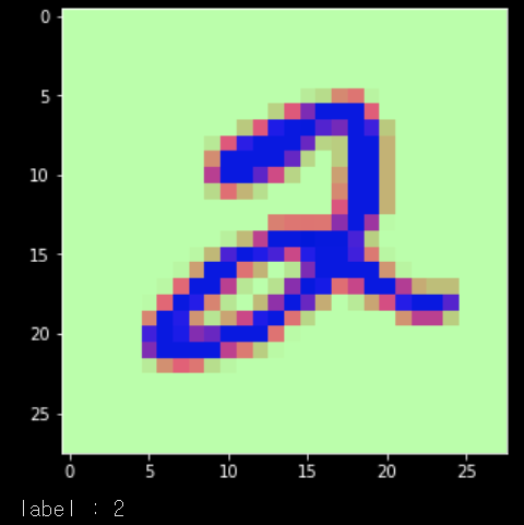
각각의 이미지는 $28 \times 28$ pixel들을 가지고 있기 때문에 우리는 $ 28 \times 28 = 784$ 차원의 백터를 가지게 됩니다. 하지만 784차원의 공간에서 우리의 MNIST가 차지하는 공간은 매우 작을 것입니다.
784차원은 굉장히 거대하고 매우매우 많은 벡터들이 존재합니다. 이해하기 쉽게 랜덤하게 하나를 뽑아서 이미지로 나타내 봅니다.
plt.clf()
plt.figure(figsize=(5,5))
rand_img = np.random.rand(28,28)
plt.imshow(rand_img)
plt.show()
이렇게 수많은 이미지들 중에 숫자를 나타내는 이미지는 매우 드물 것입니다. 그렇기 때문에 차지하는 차원도 더 작을 것입니다. 그래서 이 매우 드문 것들을 더 작은 차원으로 내리기 위해 PCA 방법을 사용해봅니다.
Step 3. Visualization using PCA
PCA는 Principal Components Analysis의 약자로, 데이터가 가장 흩어져있는 축을 찾아서 그곳으로 사영해서 원하는 차원 개수만큼 줄이는 방법입니다.
데이터가 가장 흩어져있는 축이라는 말은 가장 분산(Variance)이 커지게 하는 축이라는 말과 같습니다.
Scikit-learn 패키지를 활용해서 PCA를 이해해봅니다.
먼저 42000개의 데이터는 개수가 너무 많기 때문에 개수를 좀 줄여서 15000개를 가지고 진행합니다.
labels = y[:15000]
data = X[:15000]

print("the shape of sample data = ", data.shape)
그리고 Feature의 개수가 매우 많기 때문에 Z-Score를 사용하여 정규화를 시켜줍니다.
Scikit-learn 패키지 안의 StandardScaler 함수를 통해서 진행합니다.
from sklearn.preprocessing import StandardScaler
standardized_data = StandardScaler().fit_transform(data)

sample_data = standardized_data
이제 Scit-learn 패키지 안의 PCA 패키지를 가져와서 적용해봅니다.
from sklearn import decomposition
pca = decomposition.PCA()
2차원으로 축소를 하기 때문에 Number of Components를 2로 해줍니다.
# configuring the parameteres
# the number of components = 2
pca.n_components = 2
pca_data = pca.fit_transform(sample_data)

# pca_reduced will contain the 2-d projects of simple data
print("shape of pca_reduced.shape = ", pca_data.shape)
원래 우리가 가지고 있던 데이터는 784차원이었는데, PCA를 통해서 2로 줄어든 것을 확인할 수 있습니다.
이제 이것을 시각화해서 보도록하겠습니다. 라벨마다 색을 부여해서 시각화하겠습니다.
# attaching the label for each 2-d data point
pca_data = np.vstack((pca_data.T, labels)).T
import seaborn as sn
# creating a new data fram which help us in ploting the result data
pca_df = pd.DataFrame(data=pca_data, columns=("1st_principal", "2nd_principal", "label"))
sn.FacetGrid(pca_df, hue="label", size=6).map(plt.scatter, '1st_principal', '2nd_principal').add_legend()
plt.show()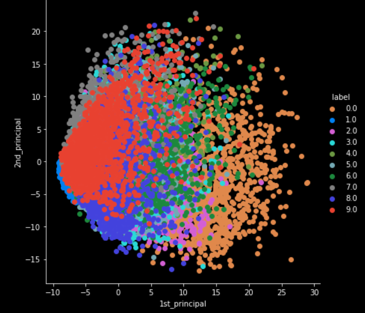
축소된 이미지를 보았을 때, 비슷한 라벨의 이미지들끼리 모여있는 것으로보아 잘 축소된 것을 알 수 있습니다.
다음은 패키지를 사용하지 않고 직접 eigen vector를 구하고, 데이터들을 사영시키면서 차원 축소를 진행해보겠습니다.
Step 4. Implement PCA
먼저, 고유값(Eigen Value)과 고유백터(Eigen Vector)를 구하기 위해서 공분산 행렬을 먼저 구합니다.
이 때 우리가 이미 Z-Score 을 해주었기 때문에 Sample_data의 평균이 0입니다. 그래서 공분산 행렬(co-variance matrix)을 구하는 식이 다음과 같이 간단해집니다.
$$Cov(X, X) = \text{E}\left(\left(X - \bar{X}\right)\left(X - \bar{X}\right)^\top\right) =\text{E}\left(XX^\top\right)$$
여기서 X는 (차원 수 x 데이터 개수)의 형태의 matrix이기 때문에 예시에서는 전치(Transpose)시켜서 진행하도록합니다.

sample_data.mean()
이제 구한 공분산 행렬을 가지고, scipy 패키지 안의 eigh 함수를 통해서 eigen value와 eigen vector를 구해봅니다. 2D로 차원을 축소할 것이기 때문에 가장 큰 두 개의 값을 선정해서 구해봅니다.
# finding the top two eigen-values and corresponding eigen-vectors
# for projecting onto a 2-Dim space.

from scipy.linalg import eigh

# the parameter 'eigvals' is defined (low value to heigh value)
# eigh function will return the eigen values in asending order
# this code generates only the top 2 (782 and 783)(index) eigenvalues.
# 아 eigval이 784개이니까(메트릭스 linearly indep 여부는? 이미 수직인 차원 다루는거라 ㄱㅊ군), 그중 제일 큰애 2개
values, vectors = eigh(covar_matrix, eigvals=(782,783))

print("Shape of eigen vectors = ",vectors.shape)
# converting the eigen vectors into (2,d) shape for easyness of further computations
vectors = vectors.T

print("Updated shape of eigen vectors = ",vectors.shape)
# here the vectors[1] represent the eigen vector corresponding 1st principal eigen vector
# here the vectors[0] represent the eigen vector corresponding 2nd principal eigen vector
이제 구한 eigen vector를 축으로 데이터를 사영시켜줍니다.
# projecting the original data sample on the plane
#formed by two principal eigen vectors by vector-vector multiplication.

import matplotlib.pyplot as plt
new_coordinates = np.matmul(vectors, sample_data.T)

print (" resultanat new data points' shape ", vectors.shape, "X", sample_data.T.shape," = ", new_coordinates.shape)
labels.shape
데이터가 784차원에서 2차원으로 줄어들었습니다.
import pandas as pd

# appending label to the 2d projected data(vertical stack)
new_coordinates = np.vstack((new_coordinates, labels.reshape(1,-1))).T

# creating a new data frame for ploting the labeled points.
dataframe = pd.DataFrame(data=new_coordinates, columns=("1st_principal", "2nd_principal", "label"))
print(dataframe.head())
#(0,1,2,3,4 are Xi other are principal axis)
각 라벨마다 색을 부여해서 시각화해봅니다.
import seaborn as sn
sn.FacetGrid(dataframe, hue="label", size=6).map(plt.scatter, '1st_principal', '2nd_principal').add_legend()
plt.show()
Scikit-learn 패키지로 구한 것과 직접 사영한 것이 비슷한 형태로 나타나는 것을 확인할 수 있습니다.