[ML 머신러닝] Multiple Linear Regression 다중 선형 회귀 분석

Multiple Linear Regression 다중 선형 회귀 분석은 Single Linear Regression과 달리 하나 이상의 다양한 변수들을 고려해서 분석하는 방식입니다. 예를 들어서 집 값을 예측하고자 한다면, 집의 크기, 주변의 편의 시설, 위치, 화장실의 개수, 건축 년도 등등 고려해야 할 것들이 매우 많습니다. 이번 과제에서는 이렇게 다양한 입력 변수들을 다루는 multiple linear regression에 대해서 알아봅니다.

Step. 1 Dataset

이번시간에는 자동차의 여러 기술적인 사양들을 고려해서 연비를 예측해보겠습니다.

Auto Miles Per Gallon(MPG) Dataset을 불러옵니다.

import pandas
import seaborn
seaborn.set()

from urllib.request import urlretrieve
URL = 'https://go.gwu.edu/engcomp6data3'
urlretrieve(URL, 'auto_mpg.csv')

mpg_data = pandas.read_csv('/content/auto_mpg.csv')
mpg_data.head()

mpg_data.info()를 통해서 Data에 대한 정보를 살펴볼 수 있습니다.

mpg_data.info()

정보들을 살펴보자면, 총 392개의 데이터가 있고 9개의 컬럼들이 있습니다.

여기서 car name은 자료형이 object 타입입니다. (사용하기 위해서는 형변환을 해주어야합니다.)

그리고 origin은 int로 정수 형태이지만, 이는 만들어진 도시로 카테고리화 한 값입니다. (ex. 서울 : 1, 경기 : 2, ...)

이러한 이유로 이번 linear regression에서는 car name과 origin은 제외하고 분석합니다.

y_col = 'mpg'
x_cols = mpg_data.columns.drop(['car name', 'origin', 'mpg'])  # also drop mpg column

Step. 2 Data exploration

우선 linear regression을 진행하기에 앞서 자동차의 정보들과 연비와의 상관관계를 알아보겠습니다.

이 때는 데이터를 시각화하는 그래프를 그리는 것이 가장 직관적으로 이해하기 좋습니다.

seaborn.pairplot(data=mpg_data, height=5, aspect=1,
             x_vars=x_cols,
             y_vars=y_col);

Accerlation과 model_year의 정보는 양의 상관관계에 있고 나머지는 음의 상관관계에 있습니다.

이러한 상관관계를 통해서 linear model이 연비를 예측하는데 충분하다는 것을 알 수 있습니다.

Step. 3 Linear model in matrix form

Multiple linear regression 에서 입력 변수가 $d$ 개라고 하면 우리가 찾아야 하는 model은 다음과 같습니다.
$\hat{y} = w_{0} + w_{1} x_{1} + w_{2} x_{2} + . . . + w_{d} x_{d}$
여기서 $\hat{y}$ 는 우리가 예측한 값입니다. 여기서 편의를 위해 $x_{0} = 1$ 를 추가해서 위 식을 정리하면 다음과 같게 됩니다.
$\hat{y} = \sum_{i = 0}^{d} w_{i} x_{i} = x^{⊤} w$
여기서 $x = (x_{0}, x_{1}, . . ., x_{d})$ 로 입력 변수들로 이루어진 벡터이고 $w = (w_{0}, w_{1}, . . ., w_{d})$ 로 입력 변수에 곱해지는 계수들로 이루어진 벡터입니다.

이제 우리는 392개의 데이터를 가지고 있습니다. 이를 $N$ 개라고 생각하고 식을 나열해보면 다음과 같습니다.
${\hat{y}}^{(1)} = w_{0} x_{0}^{(1)} + w_{1} x_{1}^{(1)} + w_{2} x_{2}^{(1)} + . . . + w_{d} x_{d}^{(1)}$
${\hat{y}}^{(2)} = w_{0} x_{0}^{(2)} + w_{1} x_{1}^{(2)} + w_{2} x_{2}^{(2)} + . . . + w_{d} x_{d}^{(2)}$
$⋮$
${\hat{y}}^{(N)} = w_{0} x_{0}^{(N)} + w_{1} x_{1}^{(N)} + w_{2} x_{2}^{(N)} + . . . + w_{d} x_{d}^{(N)}$
이제 최종적으로 위의 식을 한번에 행렬의 형태로 표현하면 다음과 같습니다.

$\hat{y} = [\begin{matrix} {\hat{y}}^{(1)} \\ {\hat{y}}^{(2)} \\ ⋮ \\ {\hat{y}}^{(N)} \end{matrix}] = [\begin{matrix} x_{0}^{(1)} & x_{1}^{(1)} & \dots & x_{d}^{(1)} \\ x_{0}^{(2)} & x_{1}^{(2)} & \dots & x_{d}^{(2)} \\ ⋮ & ⋮ & ⋱ & ⋮ \\ x_{0}^{(N)} & x_{1}^{(N)} & \dots & x_{d}^{(N)} \end{matrix}] [\begin{matrix} w_{0} \\ w_{1} \\ ⋮ \\ w_{d} \end{matrix}] = X w$

여기서 $x$ 는 입력 변수들을 행렬의 형태로 나타낸 것입니다. 그리고 맨 앞에 $x_{0} = 1$ 을 추가했었기 때문에 $X$ 의 맨 왼쪽 행렬은 1로 이루어져 있습니다.

그리고 $\hat{y}$ 는 예측한 변수들을 모아놓은 벡터이고, $y$ 는 실제 연비들을 모아놓은 벡터입니다.

이제 이것들을 코드로 표현해 보겠습니다.

from autograd import numpy
from autograd import grad

X = mpg_data[x_cols].values
X = numpy.hstack((numpy.ones((X.shape[0], 1)), X))  # pad 1s to the left of input matrix
y = mpg_data[y_col].values

print("X.shape = {}, y.shape = {}".format(X.shape, y.shape))

이제 Mean Squared Error(MSE) 를 사용해서 cost function을 정의해보겠습니다.

※ MSE는 통계적 추정의 정확성에 대한 질적인 척도로 사용하면 수학적인 분석이 쉽고 계산이 용이합니다. 또 수치가 작을 수록 정확성이 높다는 의미입니다.
$L (y, \hat{y}) = \frac{1}{N} \sum_{i = 1}^{N} (y^{(i)} - {\hat{y}}^{(i)})^{2}$
Cost function과 우리의 linear regression model을 코드로 나타내면 다음과 같습니다.

def linear_regression(params, X):
    '''
    The linear regression model in matrix form.
    Arguments:
      params: 1D array of weights for the linear model
      X     : 2D array of input values
    Returns:
      1D array of predicted values
    '''
    return numpy.dot(X, params)

def cost_function(params, model, X, y):
    '''
    The mean squared error loss function.
    Arguments:
      params: 1D array of weights for the linear model
      model : function for the linear regression model
      X     : 2D array of input values
      y     : 1D array of predicted values
    Returns:
      float, mean squared error
    '''
    y_pred = model(params, X)
    return numpy.mean( numpy.sum((y - y_pred)**2) )

Step. 4 Find the weights using gradient descent

<경사 하강법을 사용하여 가중치 찾기>

이제 Gradient descent로 cost function을 최소로 해주는 계수(weight)를 찾아보겠습니다. `autograd.grad()` 함수로 기울기를 구해서 사용하겠습니다.

gradient = grad(cost_function)

기울기 값이 잘 구해지는지 랜덤한 값을 통해 알아봅니다.

gradient(numpy.random.rand(X.shape[1]), linear_regression, X, y)

기울기 값이 매우 크게 나오는 것을 알 수 있습니다. 이상태로 한 번 gradient descent를 진행해봅니다.

max_iter = 30
alpha = 0.001
params = numpy.zeros(X.shape[1])

for i in range(max_iter):
    descent = gradient(params, linear_regression, X, y)
    params = params - descent * alpha
    loss = cost_function(params, linear_regression, X, y)
    if i%5 == 0:
        print("iteration {}, loss = {}".format(i, loss))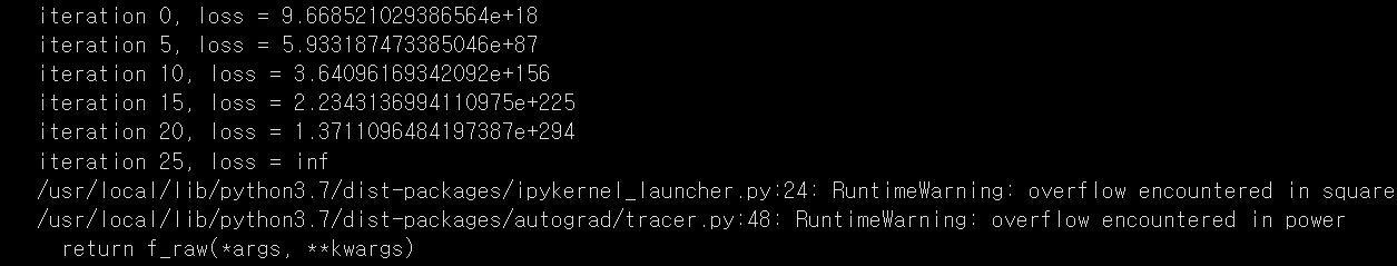

loss가 무한대를 넘어가서 오류가 발생했습니다.

Step. 5 Feature scaling

Gradient descent를 진행했더니 loss가 무한대로 발산했습니다. 이것은 입력 변수들 중에 특정 값들이 너무 커서 일어난 일입니다. 입력 데이터들의 최대값과 최소값을 출력해봅니다.

mpg_data[x_cols].describe().loc[['max', 'min']]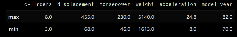

weight 값을 보면 다른 값들에 비해 매우 큰 것을 알 수 있습니다. 그래서 우리는 값들을 비슷한 크기를 가지도록 바꿔줄 필요가 있습니다. 물론 값들이 비슷한 크기를 가지게 만드는 방법 정규화(Normalization)는 데이터에 따라 여러가지 방법이 있습니다. 그 중에는 가장 큰 값을 1로 가장 최소값을 0으로 맞춰주는 방식이 있고 1과 -1로 맞춰줄 수도 있습니다. 그리고 평균과 분산을 이용하는 방식(Standardization)도 있습니다. 이번에 사용할 방법은 min-max scaling으로 모든 데이터의 범위를 최대 1, 최소 0으로 맞춰줍니다. 변환하는 방법은 다음 식과 같습니다.

$x^{'} = \frac{x - min (x)}{max (x) - min (x)}$

scikit-learn이라는 패키지를 이용해서 이러한 정규화(Normalization)를 해봅니다.

from sklearn.preprocessing import MinMaxScaler

min_max_scaler = MinMaxScaler()
X_scaled = min_max_scaler.fit_transform(mpg_data[x_cols])
X_scaled = numpy.hstack((numpy.ones((X_scaled.shape[0], 1)), X_scaled)) 

pandas.DataFrame(X_scaled).describe().loc[['max', 'min']]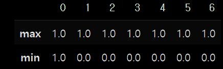

max_iter = 1000
alpha = 0.001
params = numpy.zeros(X.shape[1])

for i in range(max_iter):
    descent = gradient(params, linear_regression, X_scaled, y)
    params = params - descent * alpha
    loss = cost_function(params, linear_regression, X_scaled, y)
    if i%100 == 0:
        print("iteration {}, loss = {}".format(i, loss))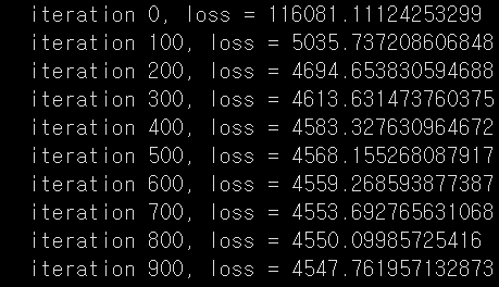

loss 값이 낮아지며 params가 학습 완료되었습니다. 학습된 params는 다음과 같고, 예측 값을 params와 $X$ 의 곱으로 나타낼 수 있습니다.

params

y_pred_gd = X_scaled @ params

Step 6. How accurate is the model?

이제 우리가 만든 모델은 얼마나 정확할까요? Regression에서는 주로 두 개의 기본 지표가 있습니다. Mean Absolute Error(MAE)와 Root Mean Squared Error(RMSE)입니다. 참고로 RMSE는 아까 만든 Cost function에 Root를 씌어준 것입니다.

두 개의 식은 아래와 같습니다.

$MAE (y, \hat{y}) = \frac{1}{N} \sum_{i = 1}^{N} | y^{(i)} - {\hat{y}}^{(i)} |$
$RMSE (y, \hat{y}) = \sqrt{\frac{1}{N} \sum_{i = 1}^{N} (y^{(i)} - {\hat{y}}^{(i)})^{2}}$

이 지표들도 scikit-learn 패키지를 통해서 만들어봅니다.

from sklearn.metrics import mean_absolute_error, mean_squared_error

mae = mean_absolute_error(y, y_pred_gd)
rmse = mean_squared_error(y, y_pred_gd, squared=False)
print("mae  = {}".format(mae))
print("rmse = {}".format(rmse))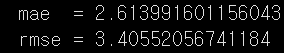

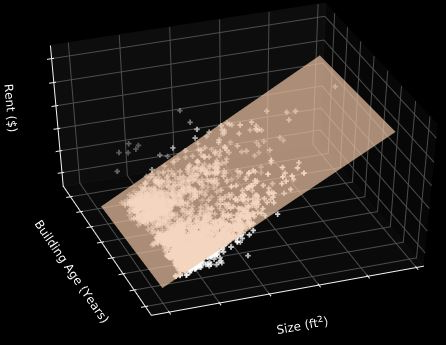
잠깐✋> 왜 Multiple Linear Regression에서는 결과물을 그래프로 시각화하지 않을까요?

그 이유는 변수들이 많아지면서 그래프가 3차원을 넘어가면, 인간의 인지능력으로는 인지할 수 없어지기 때문입니다.

※ 참고로 3차원 상에서 Linear Regression 그래프는 아래와 같이 그려집니다.

저작자표시 비영리 변경금지

일	월	화	수	목	금	토
		1	2	3	4	5
6	7	8	9	10	11	12
13	14	15	16	17	18	19
20	21	22	23	24	25	26
27	28	29	30

내 블로그 - 관리자 홈 전환	`Q` `Q`
새 글 쓰기	`W` `W`

글 수정 (권한 있는 경우)	`E` `E`
댓글 영역으로 이동	`C` `C`

이 페이지의 URL 복사	`S` `S`
맨 위로 이동	`T` `T`
티스토리 홈 이동	`H` `H`
단축키 안내	`Shift` + `/` `⇧` + `/`

고양이의 알쏭달쏭 공부방

[ML 머신러닝] Multiple Linear Regression 다중 선형 회귀 분석

Step. 1 Dataset

Step. 2 Data exploration

Step. 3 Linear model in matrix form

Step. 4 Find the weights using gradient descent

Step. 5 Feature scaling

Step 6. How accurate is the model?

티스토리툴바

단축키

내 블로그

블로그 게시글

모든 영역