이전에 [ML 머신러닝]에서 했던 학습들은 전부 레이어(Layer)를 하나만 쌓아서 학습했습니다. 이번 장에서는 Layer의 개수를 1개 더 늘려서 성능이 올라가는지 확인해보겠습니다. Layer를 하나 쌓아서 학습하는 LR(Linear regression)과 non-linear를 추가해서 layer 2개를 쌓아서 만든 MLP(Multi-Layer Percaptron)를 만들어 비교해보겠습니다. 전장에서 사용했던 Metal-Casting Parts dataset을 활용해서 진행해봅니다.
Step 1. Images of Metal-Casting Parts
필요한 모듈과 데이터를 불러옵니다.
from autograd import numpy
from autograd import grad
from matplotlib import pyplot
from urllib.request import urlretrieve
URL = 'https://github.com/engineersCode/EngComp6_deeplearning/raw/master/data/casting_images.npz'
urlretrieve(URL, 'casting_images.npz')

# read in images and labels
with numpy.load("/content/casting_images.npz", allow_pickle=True) as data:
    ok_images = data["ok_images"]
    def_images = data["def_images"]
데이터를 확인해줍니다.
n_ok_total = ok_images.shape[0]
res = int(numpy.sqrt(def_images.shape[1]))

print("Number of images without defects:", n_ok_total)
print("Image resolution: {} by {}".format(res, res))
n_def_total = def_images.shape[0]
print("Number of images with defects:", n_def_total)fig, axes = pyplot.subplots(2, 3, figsize=(8, 6), tight_layout=True)
axes[0, 0].imshow(ok_images[0].reshape((res, res)), cmap="gray")
axes[0, 1].imshow(ok_images[50].reshape((res, res)), cmap="gray")
axes[0, 2].imshow(ok_images[100].reshape((res, res)), cmap="gray")
axes[1, 0].imshow(ok_images[150].reshape((res, res)), cmap="gray")
axes[1, 1].imshow(ok_images[200].reshape((res, res)), cmap="gray")
axes[1, 2].imshow(ok_images[250].reshape((res, res)), cmap="gray")
fig.suptitle("Casting parts without defects", fontsize=20);fig, axes = pyplot.subplots(2, 3, figsize=(8, 6), tight_layout=True)
axes[0, 0].imshow(def_images[0].reshape((res, res)), cmap="gray")
axes[0, 1].imshow(def_images[50].reshape((res, res)), cmap="gray")
axes[0, 2].imshow(def_images[100].reshape((res, res)), cmap="gray")
axes[1, 0].imshow(def_images[150].reshape((res, res)), cmap="gray")
axes[1, 1].imshow(def_images[200].reshape((res, res)), cmap="gray")
axes[1, 2].imshow(def_images[250].reshape((res, res)), cmap="gray")
fig.suptitle("Casting parts with defects", fontsize=20);Step 2. Split Dataset
학습과 평가를 위한 dataset으로 나눕니다.
# numbers of images for validation (~ 20%)
n_ok_val = int(n_ok_total * 0.2)
n_def_val = int(n_def_total * 0.2)
print("Number of images without defects in validation dataset:", n_ok_val)
print("Number of images with defects in validation dataset:", n_def_val)

# numbers of images for test (~ 20%)
n_ok_test = int(n_ok_total * 0.2)
n_def_test = int(n_def_total * 0.2)
print("Number of images without defects in test dataset:", n_ok_test)
print("Number of images with defects in test dataset:", n_def_test)

# remaining images for training (~ 60%)
n_ok_train = n_ok_total - n_ok_val - n_ok_test
n_def_train = n_def_total - n_def_val - n_def_test
print("Number of images without defects in training dataset:", n_ok_train)
print("Number of images with defects in training dataset:", n_def_train)
numpy 패키지 안에 있는 split 함수로 나누어줍니다.
ok_images = numpy.split(ok_images, [n_ok_val, n_ok_val+n_ok_test], 0)
def_images = numpy.split(def_images, [n_def_val, n_def_val+n_def_test], 0)
numpy 패키지 안에 있는 concatenate 함수를 이용해서 train, val, test끼리 결함이 있는 이미지와 없는 이미지들을 합쳐줍니다.
images_val = numpy.concatenate([ok_images[0], def_images[0]], 0)
images_test = numpy.concatenate([ok_images[1], def_images[1]], 0)
images_train = numpy.concatenate([ok_images[2], def_images[2]], 0)
Step. 3 Data Normalization : Z-Score Normalization
Z-Score를 이용하여 Train, Validation, Test 데이터를 정규화 합니다.
images_train.max(), images_train.min()
# calculate mu and sigma
mu = numpy.mean(images_train, axis=0)
sigma = numpy.std(images_train, axis=0)

# normalize the training, validation, and test datasets
images_train = (images_train - mu) / sigma
images_val = (images_val - mu) / sigma
images_test = (images_test - mu) / sigmaimages_train.max(), images_train.min()
데이터를 확인해보면 255->7.xxx로 1 -> -4.xxx로 정규화 된것을 확인할 수 있습니다.
Step 4. Creating Labels and Classes
데이터셋에 Class Labels을 정해주어야 합니다. 즉, 이 이미지가 결함이 있는지 없는지 명시적으로 나타내주는 것입니다.
결함이 있는 것을 1로, 없는 것을 0으로 라벨링(labeling)해줍니다.
# labels for training data
labels_train = numpy.zeros(n_ok_train+n_def_train)
labels_train[n_ok_train:] = 1.

# labels for validation data
labels_val = numpy.zeros(n_ok_val+n_def_val)
labels_val[n_ok_val:] = 1.

# labels for test data
labels_test = numpy.zeros(n_ok_test+n_def_test)
labels_test[n_ok_test:] = 1.
입력으로 들어온 이미지에 결함이 있는지 없는지 알아내기 위해 Logistic Model을 사용합니다.
def classify(x, model, params):
    """Use a logistic model to label data with 0 or/and 1.

    Arguments
    ---------
    x : numpy.ndarray
        The input of the model. The shape should be (n_images, n_total_pixels).
    params : a tuple/list of two elements
        The first element is a 1D array with shape (n_total_pixels). The
        second element is a scalar.

    Returns
    -------
    labels : numpy.ndarray
        The shape of the label is the same with `probability`.

    Notes
    -----
    This function only works with multiple images, i.e., x has a shape of
    (n_images, n_total_pixels).
    """
    probabilities = model(x, params)
    labels = (probabilities >= 0.5).astype(float)
    return labels
출력 확률 값이 0.5보다 크면 결함이 있고, 0.5보다 작으면 결함이 없다고 하는 classify 함수를 만들었습니다.
Step 5. Evaluating Model Performance
이제 학습한 모델이 얼마나 잘 예측을 하는지 알아봅니다.
모델이 예측한 결과는 다음 4가지 종류로 분류할 수 있습니다.
- True Positive(TP) : 결함이 있다고 예측한 것들 중 실제로 결함이 있는 것
- False Positive(FP) : 결함이 있다고 예측한 것들 중에서 실제로 결함이 없는 것
- True Negative(TN) : 결함이 없다고 예측한 것들 중에서 실제로 결함이 없는 것
- False Negative(FN) : 결함이 없다고 예측한 것들 중에서 실제로 결함이 있는 것
| 결함이 있다고 예측 | 결함이 없다고 예측 | |
| 실제로 결함이 있음 | ||
| 실제로 결함이 없음 |
위에서
이제 위에서 설명한 것들을 가지고 가장 보편적으로 사용하는 지표 3가지를 알아보도록 하겠습니다.
여기서 정밀도(Precision)와 재현율(Recall)로 F-score를 계산할 수 있습니다.
정밀도(Precision)와 재현율(Recall) 사이에 우선순위를 정하는 것은 매우 중요한 작업입니다.
예를들어 CT 촬영 데이터를 가지고 암진단을 한다고 가정해봅니다. 실제로 암에 걸렸는데 안걸렸다고 판정하는것과 암에 안걸렸는데 걸렸다고 판정하는 것 두 가지중 어떤 것이 더 위험할까요?
환자가 암에 걸렸는데 안걸렸다고 판단을 내리는 것이 훨씬 위험할 것입니다. 이처럼 모델이 어떻게 사용되느냐에 따라서 둘 사이의 우선순위를 결정하는 것은 매우 중요한 일이 됩니다.
이제 accuracy와 f1-score을 구하는 함수를 코드로 작성해봅니다.
def performance(predictions, answers, beta=1.0):
    """Calculate precision, recall, and F-score.

    Arguments
    ---------
    predictions : numpy.ndarray of integers
        The predicted labels.
    answers : numpy.ndarray of integers
        The true labels.
    beta : float
        A coefficient representing the weight of recall.

    Returns
    -------
    precision, recall, score, accuracy : float
        Precision, recall, and F-score, accuracy respectively.
    """
    true_idx = (answers == 1)  # the location where the answers are 1
    false_idx = (answers == 0)  # the location where the answers are 0

    # true positive: answers are 1 and predictions are also 1
    n_tp = numpy.count_nonzero(predictions[true_idx] == 1)

    # false positive: answers are 0 but predictions are 1
    n_fp = numpy.count_nonzero(predictions[false_idx] == 1)

    # true negative: answers are 0 and predictions are also 0
    n_tn = numpy.count_nonzero(predictions[false_idx] == 0)

    # false negative: answers are 1 but predictions are 0
    n_fn = numpy.count_nonzero(predictions[true_idx] == 0)

    # precision, recall, and f-score
    precision = n_tp / (n_tp + n_fp)
    recall = n_tp / (n_tp + n_fn)
    score = (
        (1.0 + beta**2) * precision * recall /
        (beta**2 * precision + recall)
    )

    accuracy = (n_tp + n_tn) / (n_tp + n_fn + n_fp + n_tn)

    return precision, recall, score, accuracy
Step 6. Model
Logistic regression과 2 Layers MLP model을 구현해봅니다.
def logistic(x):
    """Logistic/sigmoid function.

    Arguments
    ---------
    x : numpy.ndarray
        The input to the logistic function.

    Returns
    -------
    numpy.ndarray
        The output.

    Notes
    -----
    The function does not restrict the shape of the input array. The output
    has the same shape as the input.
    """

    return 1. / (1. + numpy.exp(-x))
로지스틱(시그 모이어) 함수입니다.
def LR_model(x, params):
    """A logistic regression model.

    A logistic regression is y = sigmoid(x * w + b), where the operator *
    denotes a mat-vec multiplication.

    Arguments
    ---------
    x : numpy.ndarray
        The input of the model. The shape should be (n_images, n_total_pixels).
    params : a tuple/list of two elemets
        The first element is a 1D array with shape (n_total_pixels). The
        second element is a scalar (the intercept)

    Returns
    -------
    probabilities : numpy.ndarray
        The output is a 1D array with length n_samples.
    """

    return logistic(numpy.dot(x, params[0]) + params[1])
로지스틱 함수(Logistic Regression)를 사용한 LR 모델입니다.
def MLP_model(x, params):
    """ A MLP model.

    A MLP is y = sigmoid(max((x * w1 + b1), 0) *w2 +b2), where the operator *
    denotes a mat-vec multiplication.
    Arguments
    ---------
    x : numpy.ndarray
        The input of the model. The shape should be (n_images, n_total_pixels).
    params : a tuple/list of four elemets
        The first element is a 1D array with shape (n_total_pixels). The
        second element is a scalar (the intercept)

    Returns
    -------
    probabilities : numpy.ndarray
        The output is a 1D array with length n_samples.
    """
    x = numpy.dot(x, params[0]) + params[1]
    x = numpy.maximum(x, 0)

    return logistic(numpy.dot(x, params[2]) + params[3])
레이어를 한 개 더 쌓은 MLP 모델입니다.
다음은 cost function을 만들어줍니다. Logistic regression장에서 사용했던 cost function을 다시 사용하겠습니다.
이것을 벡터꼴로 나타내면 다음과 같습니다.
코드로 구현해봅니다.
def model_loss(x, true_labels, model, params):
    """Calculate the predictions and the loss w.r.t. the true values.

    Arguments
    ---------
    x : numpy.ndarray
        The input of the model. The shape should be (n_images, n_total_pixels).
    true_labels : numpy.ndarray
        The true labels of the input images. Should be 1D and have length of
        n_images.
    params : a tuple/list of two elements
        The first element is a 1D array with shape (n_total_pixels). The
        second elenment is a scalar.

    Returns
    -------
    loss : a scalar
        The summed loss.
    """

    pred = model(x, params)

    loss = - (
        numpy.dot(true_labels, numpy.log(pred+1e-15)) +
        numpy.dot(1.-true_labels, numpy.log(1.-pred+1e-15))
    )

    return loss
Step 7. Initialization
LR과 MLP에서 사용할 Parameter들을 초기화합니다.
# a function to get the gradients of a logistic model
gradients = grad(model_loss, argnum=3)

# initialize LR parameters
std = 1e-4
LR_w = std * numpy.random.randn(images_train.shape[1])
LR_b = numpy.zeros(1)

# initialize MLP parameters
hidden = 32
w0 = std * numpy.random.randn(images_train.shape[1], hidden)
b0 = numpy.zeros(hidden)
w1 = std * numpy.random.randn(hidden)
b1 = numpy.zeros(1)
Step 8. Training / Optimization
두 모델을 학습하고, 최적화시킨 후 성능을 비교해봅니다.
총 5000번 학습을 하는 동안 가장 높은 정확도(Accuracy)를 측정해줍니다.
먼저 일반 Logistic Regression(LR) 모델입니다.
# learning rate
lr = 1e-5

# a variable for the change in validation loss
change = numpy.inf

# a counter for optimization iterations
i = 0

# a variable to store the validation loss from the previous iteration
old_val_loss = 1e-15
best_acc = 0.0
# keep running if:
#   1. we still see significant changes in validation loss
#   2. iteration counter < 10000
while i < 5000:

    # calculate gradients and use gradient descents
    grads = gradients(images_train, labels_train, LR_model, (LR_w, LR_b))
    LR_w -= (grads[0] * lr)
    LR_b -= (grads[1] * lr)

    # validation loss
    val_loss = model_loss(images_val, labels_val, LR_model, (LR_w, LR_b))

    # calculate f-scores against the validation dataset
    pred_labels_val = classify(images_val, LR_model, (LR_w, LR_b))
    score = performance(pred_labels_val, labels_val)
    best_acc = max(best_acc, score[3])
    # calculate the chage in validation loss
    change = numpy.abs((val_loss-old_val_loss)/old_val_loss)

    # update the counter and old_val_loss
    i += 1
    old_val_loss = val_loss

    # print the progress every 10 steps
    if i % 10 == 0:
        print("{}...".format(i), end="")

score = performance(pred_labels_val, labels_val)
print("")
print("")
print("Upon optimization stopped:")
print("    Iterations:", i)
print("    Best Accuracy:", best_acc)
MLP 모델입니다.
# learning rate
lr = 1e-5

# a variable for the change in validation loss
change = numpy.inf

# a counter for optimization iterations
i = 0

# a variable to store the validation loss from the previous iteration
old_val_loss = 1e-15
best_acc = 0.0

# keep running if:
#   1. we still see significant changes in validation loss
#   2. iteration counter < 10000
while i < 5000:

    # calculate gradients and use gradient descents
    grads = gradients(images_train, labels_train, MLP_model, (w0, b0, w1, b1))
    w0 -= (grads[0] * lr)
    b0 -= (grads[1] * lr)
    w1 -= (grads[2] * lr)
    b1 -= (grads[3] * lr)

    # validation loss
    val_loss = model_loss(images_val, labels_val, MLP_model, (w0, b0, w1, b1))

    # calculate f-scores against the validation dataset
    pred_labels_val = classify(images_val, MLP_model, (w0, b0, w1, b1))
    score = performance(pred_labels_val, labels_val)
    best_acc = max(best_acc, score[3])
    # calculate the chage in validation loss
    change = numpy.abs((val_loss-old_val_loss)/old_val_loss)

    # update the counter and old_val_loss
    i += 1
    old_val_loss = val_loss

    # print the progress every 10 steps
    if i % 10 == 0:
        print("{}...".format(i), end="")

score = performance(pred_labels_val, labels_val)
print("")
print("")
print("Upon optimization stopped:")
print("    Iterations:", i)
print("    Best Accuracy:", best_acc)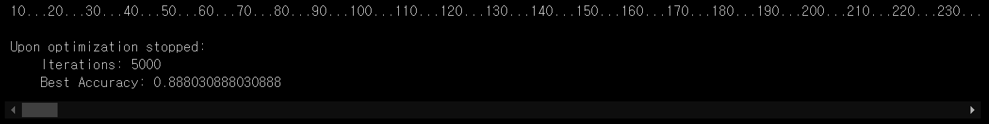
실재로 측정 결과 MLP 모델이 LR 모델보다 더 높은 정확도(Accuracy)가 나왔습니다.
Layer의 개수가 많아지고, 사이에 비선형함수(Non-Linear Function)이 추가되면, Linear한 관계만 모델링하던 LR 모델보다 더 다양하고 복잡한 함수를 모델링 할 수 있게 됩니다. 그 결과로 데이터를 잘 설명 할 수 있게 되고, 더 높은 정확도(Accuracy)를 가질 수 있게 됩니다.
더 많은 Layer를 쌓고 추가 실험을 하면서 정확도(Accuracy)도 한 번 비교해보세요!